SECURITY VALUATION
Financial Instruments such as securities (ordinary shares, preferences shares, straight bonds, convertible bonds, options) can be quoted (with a trading price) or unquoted. This section will focus on unquoted securities that are part of the capital structure of private entities and how their intrinsic value can be estimated (the Business Valuation section focuses on the intrinsic value of the whole business, as well as the equity value and value per ordinary share). The fair value of an instrument (a market-based price receivable in an orderly transaction between market participants) may be the same as its intrinsic valuation. Pricing methods will usually involve discounting techniques (shares, straight bonds) as well as option pricing models (convertibles, options).
SECURITY VALUATION: Using the Option Pricing Method for Complex Capital Structures
SECURITY VALUATION: Convertible Bond Pricing
SECURITY VALUATION: Option Pricing
SECURITIES WITH EMBEDDED OPTIONS
Security Valuation - Using the Option Pricing Method for complex capital structures
The Enterprise-Equity Value ‘Bridge’ (‘Business Valuation – Part 1: Cash Flows and Value’) may include financial instruments, other than straight debt, that have different rights attached to them. This article illustrates how various terms in financial contracts affect the fair value estimated for each tranche of instrument. It shows one method, the Option Pricing Method, to allocate enterprise value across the different instruments, using valuation techniques developed for stock option pricing (the Black-Scholes mode).
Convertible instruments and options may have been issued or granted. These allow the holder to convert into equity or exercise options to purchase equity, effecting the fair value per share of each existing ordinary shareholder due to dilution. As the enterprise value increases, options embedded in financial contracts become more attractive, making it economically worthwhile at some level to convert or exercise. The points at which these decisions are made are called ‘Breakpoints’ (the point of indifference between exercising and not-exercising rights) and the framework used a ‘Waterfall’ analysis. A hypothetical value realisable on a ‘Liquidity Event’ (‘exit’ proceeds arising on a trade sale or Initial Public Offering) can be used as the enterprise value.
Preference shares may have the following rights:
- ‘Liquidation Preference’ (‘LP’): rights that allow the holder to receive, in priority to any ordinary shareholder, a portion of the exit proceeds up to the amount of, or a multiple of, the capital they have invested. Some preference shares may have seniority over others, allowing them to rank first when the LP amount is paid out. Accrued preference dividends may also be included.
- Conversion rights: the preference shareholder may also have the right to convert their preference shares into ordinary shares at a stated ‘Conversion Ratio’, giving them an unrestricted payout as exit value increases, as well as downside protection (via their LP).
- Participation rights: these allow the holder to convert and keep their LP rights (receive the LP amount and convert), making them more valuable than non-participating preference shares, where the holder has to choose whether to convert or receive the LP amount.
Restrictions may be imposed by the founders or existing controlling shareholders in the form of:
- A Participation ‘Cap’ that limits the total payout (LP amount and share of equity proceeds on conversion), based on a multiple of the initial investment
- Mandatory Conversion at some stage exit value may force holders to convert at below their optimal level
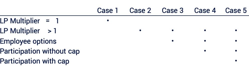
In this article, Breakpoint analysis is carried out under different scenarios building up from the base case 1:
The first breakpoint will be the LP amount or the first tranche of LP seniority (assuming no debt, which would come first). Above this point, the marginal allocation of exit proceeds changes and ordinary shareholders will start to receive value for their shares (exit value in excess of LP amount). Convertible holders will check the payout on conversion to their LP amount alternative. Option holders will exercise when their share of the exit proceeds is at least equal to the cost of exercising. Each time a convertible holder converts, their LP amount will be ignored in any subsequent calculation, unless they are participating.
The procedure used in this article checks the order of conversion and exercising in steps to determine the optimal order by seeing how other investors would react as each conversion or exercise is made (which might change the order). A good example is shown on Professor Jiro Kondo’s youtube channel (https://www.youtube.com/watch?v=b0KaBln94XI).
The equity value at any breakpoint will equal the enterprise value at that point less the remaining LP amount to be paid plus the proceeds from any options exercised. Convertible holders will convert (and forego the LP amount if non-participating) at the following equity value per share or share price (P):
P = LP per preference share / CR
= CP x LP multiple
Where:
- LP per preference share = the initial price paid for each preference share x the LP multiple
- CR = Conversion Ratio (ordinary shares received for each preference share)
- CP = Conversion Price (the initial price paid for each preference share / CR
Once the breakpoints have been established, the waterfall analysis across all breakpoints can be performed (financial instruments with proceeds/value received at each breakpoint). The Black-Scholes Model is then used to value the incremental option value at each breakpoint, taking the equity value (share price equivalent) as the maximum exit value at the final breakpoint and the exercise price as the the value at each breakpoint. This model gives call values and it is the increase in the call value at each breakpoint that is allocated to holders who receive value in that tranche based on their shareholdings. The total incremental call value allocated to each instrument over all breakpoints is the fair value of the instrument.
Security Valuation - Convertible Bond Pricing
Convertible bonds are financial instruments that entitle a holder to receive periodic interest payments (‘Coupons’) and the redemption amount (either at maturity or when the bonds are ‘Called’ by the issuer and redeemed early) - features founds in any straight bond – and that also give them the right to convert each bond into a stated number of the issuer’s ordinary shares (at the ‘Conversion Ratio’ / ‘CR’). The opportunity to receive an unlimited payoff after conversion means the coupon rate can be set lower than a straight bond. The Fair Value (‘FV’) of the bond will represent the value of the bond as straight debt plus an additional value from the conversion option. It can be estimated using option pricing methods, such as the Binomial option pricing model discussed in the article ‘Security Valuation – Option Pricing’. Conversion into equity is effectively the same as the exercise of a Call Option, where the right to convert is exercised by exchanging debt (rather than cash) for equity.
As for options, the convertible Binomial approach starts by projecting forward the share price over each time step to the final maturity period. This gives the ‘Conversion Value’ at each node (= CR x share price), being the value of shares received if converted. The value of the bond at any time step without any conversion option (its value as straight debt or ‘Investment Value’) is calculated by working back from the maturity date, first discounting the redemption amount plus final coupon at the credit risk adjusted discount rate for the final period, then discounting this value back plus the coupon at the discount rate for the penultimate period etc. In the example shown in this article, it is assumed the risk adjusted discount rate is constant, but in practice it could be assumed to vary.
At the final maturity date, the convertible will be converted or redeemed, which ever gives a higher value, so the convertible FV will equal the Conversion Value (higher share prices) or Investment Value’ (lower share prices). Like the calculation for Investment Value, the convertible FV at maturity is discounted back over the final period at some discount rate and the coupon is added to give the value of the bond at the penultimate period if held to maturity (the ‘Continuing Value’ or ‘Rollback Value’). However, the convertible FV at this penultimate date will be the greater of the Conversion Value, Investment Value and this Rollback Value. This FV is then discounted back and the recursive procedure continues back to the valuation date (root node at T=0).
There are two complications (discussed and modelled in the article):
- An issuer will usually be given the right to redeem the bonds early (‘Call’) in order to refinance the debt at a lower cost if market yields have fallen or, most likely, to control the timing of conversion to equity (‘Forced’ conversion). The convertible FV will then be: MAX ( Conversion Value, MIN {Rollback Value + coupon, Call Price + coupon} ). A coupon would not normally be paid on conversion.
- As the convertible FV at any node will reflect the value of equity, straight debt or both, when discounting back to calculate the Rollback Value a risk free rate must be applied to the equity component and the credit risk adjusted rate to the debt component. This is done by either separating out each component and discounting them accordingly, or, as in the example in this article, applying a blended discount rate that incorporates the risk free and risk adjusted rates using a probability of conversion.
Under IAS 32, the initial recognition of a convertible in the issuer’s financial statements will require separation of the liability (bond Investment Value) and equity (convertible FV less Investment Value) components (embedded call options must also be separated). The debt component should be recognised as a liability, measured at amortised cost, and the equity component as equity (if it meets the equity definition).
Security Valuation - Option Pricing
This article introduces basic option features and pricing methods (‘Binomial Model’ / ‘BM’, ‘Black-Scholes Model’ / ‘BSM’, ‘Monte Carlo’ simulation / ‘MC’), and discusses how the models can be applied when valuing employee stock options for recognition in the financial statements under International Financial Reporting Standards. No advanced maths knowledge is required to understand what options are and the general approach taken by these models when estimating Fair Value (‘FV’).
Owning an option, purchased by paying a ‘Premium’ (the option FV), entitles a holder to acquire (‘Call’ option / ‘CO’) or sell (‘Put’ option / ‘PO’) an underlying asset for a fixed amount (‘Strike’ or ‘Exercise’ price / ‘X’). If the asset market price (share price, ‘S’) increases above X, a CO is ‘in-the-money’ and an overall profit can be made if this excess exceeds the premium paid (conversely a PO holder benefits if S falls below X). An option can be exercised before the expiry (‘American’ option) or only at expiry (‘European’ option). At any exercise date, the ‘Intrinsic Value’ / ‘IV’ is the amount the option is in-the-money: S – X for a CO and X – S for a PO (nil if negative, when the option would not be exercised). This article discusses COs.
At any valuation date, the option FV should equal IV at that date plus the present value (‘PV’) of any expected increase in IV over time (‘Time Value’) as S follows an assume path until expiry. For a European option, the value depends on the expected payoff on expiry; for an American option, it might be optimal to exercise early (but only if dividends are paid on the underlying share – a European and American option will have the same value in the absence of dividends).
An option pricing model calculates the PV of the payoff (ignoring negative payoffs when the option would lapse), assuming stock prices behave according to an assumed probability distribution (the Binomial Distribution for BM, the Lognormal Distribution for BSM). The models take different approaches to forecasting stock prices, whether ‘jumping’ up or down over some ‘discrete’ time interval (day, week, month etc) (BM) or continuously changing (BSM, MC).
At any given date ti the BM assumes the stock price will increase or decrease over the next time step to ti+1 by constant factors (u and d), such that the paths recombine (a price can be reached by increasing or decreasing a prior period price). At any time period there will be t + 1 nodes, where t is the time period, with the binomial probability at each time period summing to 1. At expiry, at each node the CO value will equal the IV (max {0, S – X}) and at each prior period node it will equal the probability weighted CO value at the next period discounted at the risk free rate of interest, or, if greater, the IV at that date (if the option can be exercised).
The BSM is derived by constructing a riskless portfolio, which allows the risk free rate to be used when calculating the PV; the BM adjusts the true probabilities to risk-neutral probabilities. As the number of discrete time steps used in the BM increases, the option value converges to the continuous time BSM value.
Call Options may be granted to employees as part of their remuneration, with or without ‘vesting’ conditions that need to be fulfilled before the option ‘vests’. Under IFRS 2, the FV of the stock option is measured at the grant date and is not subsequently re-valued. The option FV is expensed to profit and loss over the vesting period (with a corresponding increase in equity), depending on the proportion of options expected to vest. The BM or BSM can be used to estimate FV, however there are some additional factors to consider.